Simulating surface codes using stim

Simulating surface codes using `stim`#

So far, you have learned about the surface code, its stabilizers and logical operators, and the effect of errors on the code. You have also learned about the Minimum-Weight Perfect Matching (MWPM) decoder for the surface code.

In this chapter, you will learn how to simulate the performance of the surface code under varying levels of physical noise using stim. As you may have noticed when we did this for repetition codes, building the syndrome extraction circuits manually is an arduous task. Many nuances need to be considered, such as avoiding qubit conflicts from overlapping parity checks and optimizing the circuit for fast execution. As you have seen in the previous chapter, even the smallest distance-3 surface codes have dense syndrome extraction circuits. stim handles this complexity automatically and makes the simulations easy to run.

In addition to the syndrome extraction circuits, we also need a fast decoder to detect and correct errors across varying distances. In the code below, we achieve all of this in just a few lines by using stim for fast circuit simulation and PyMatching (for decoding).

Step 1: Generating the circuits#

Here we choose rotated surface code measured in the \(X\)-basis. As previously discussed, the rotated variant of the surface code requires fewer physical qubits per logical qubit and is therefore better suited for execution on real quantum computers.

Unlike the case of the repetition codes, where our intent was to match stim’s results with our manually inserted noise models, we choose a more elaborate noise model that accounts for depolarization (randomly selected \(X\), \(Y\) and \(Z\) gates) after Clifford gates, and before syndrome check rounds. We also consider unintended flip errors after the initialization resets, and before measurements. While we set all these error probabilities to the same value, the component of each one is typically adjusted to fit experimental data measured directly from qubits using benchmarking techniques.

Note that we are allowing for measurement errors of the syndromes. For this reason, it’s important to capture these errors by doing more than one round – as is typical in the literature, we set the number of rounds equal to the distance.

The simulation that we are running is known as a memory experiment in the literature, since we initialize a logical state and check whether it has changed (due to an error) after some number of rounds.

p = 0.003
circuit_initial = stim.Circuit.generated("surface_code:rotated_memory_x", 
                                        distance=3, 
                                        rounds=3, 
                                        after_clifford_depolarization=p,
                                        before_round_data_depolarization=p,
                                        after_reset_flip_probability=p,
                                        before_measure_flip_probability=p)

Step 2: Generating a detector error model for the circuits#

Next, we generate the Detector Error Model (DEM) in stim. Recall the description of DEMs from our discussion implementing repetition codes in stim, where you learned that it contains the impact of the errors at various locations throughout the circuit on the detectors within the circuit.

Notice, we set decompose_errors=True as we are using a graph-based decoder. In cases where an error can trigger more than two detectors (forming a hyperedge), stim decomposes all the error mechanisms to \(\textit{edge-like}\) error mechanisms.

model = circuit_initial.detector_error_model(decompose_errors=True)

Step 3: Setting up a MWPM decoder from the DEM#

The detector error model is the input to the decoder, which in this case is PyMatching.

matching = Matching.from_detector_error_model(model)

Step 4: Run the circuits and collect the syndromes (and observable flips)#

Now, we need to sample, say, 100,000 shots from each circuit. This will allow us to see errors of order 1 in \(10^5\). Each shot will contain detector measurements, and the logical observable outcomes.

n_shots = 100_000
sampler = circuit_initial.compile_detector_sampler()
syndrome, actual_observables = sampler.sample(shots=n_shots, separate_observables=True)

Step 5: Decode the syndromes#

Next, we input the syndromes to the PyMatching decoder.

predicted_observables = matching.decode_batch(syndrome)

Step 6: Determine whether our decoder was successful#

To calculate the logical error probability, we compare the predicted outcomes from PyMatching to the actual observables. When they do not match, we will not be able to detect that the error has occurred, and a logical error results. By tracking the total number of times that the decoder failed to predict an error, we determine the logical error probability. Note that we have assumed perfect correction when the decoder successfully identifies errors in this simulation.

log_errors = []
logical_error_probability = []
num_errors = np.sum(np.any(predicted_observables != actual_observables, axis=1))
log_errors.append(num_errors/n_shots)
logical_error_probability.append(np.array(log_errors))

Putting it all together#

Now, let’s put all the pieces above together to simulate the performance of the surface code for different distances and physical error probabilities.

num_shots = 200_000
distances = [3,5,7,9,11]
physical_error_probabilities = np.logspace(-4, -1, 20)
logical_error_probabilities = []
for distance in distances:
    print(f"Simulating distance-{distance} surface codes")
    logical_errors = []
    for p in tqdm(physical_error_probabilities):
        circuit = stim.Circuit.generated("surface_code:rotated_memory_x", 
                                        distance=distance, 
                                        rounds=distance, 
                                        after_clifford_depolarization=p,
                                        before_round_data_depolarization=p,
                                        after_reset_flip_probability=p,
                                        before_measure_flip_probability=p)
        model = circuit.detector_error_model(decompose_errors=True)
        matching = Matching.from_detector_error_model(model)
        sampler = circuit.compile_detector_sampler()
        syndrome, actual_observables = sampler.sample(shots=num_shots, separate_observables=True)
        predicted_observables = matching.decode_batch(syndrome)
        num_errors = np.sum(np.any(predicted_observables != actual_observables, axis=1))
        logical_errors.append(num_errors/num_shots)
    logical_error_probabilities.append(np.array(logical_errors))

plot_logical_error_probabilities(distances = distances, 
                                 physical_errors = physical_error_probabilities, 
                                 all_logical_errors = logical_error_probabilities,
                                 all_analytical_errors=None, ylim = [1e-4, 1.1])

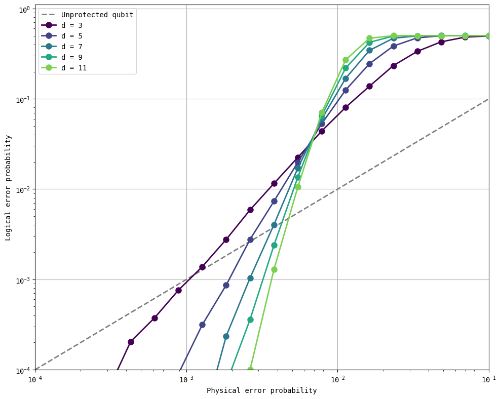
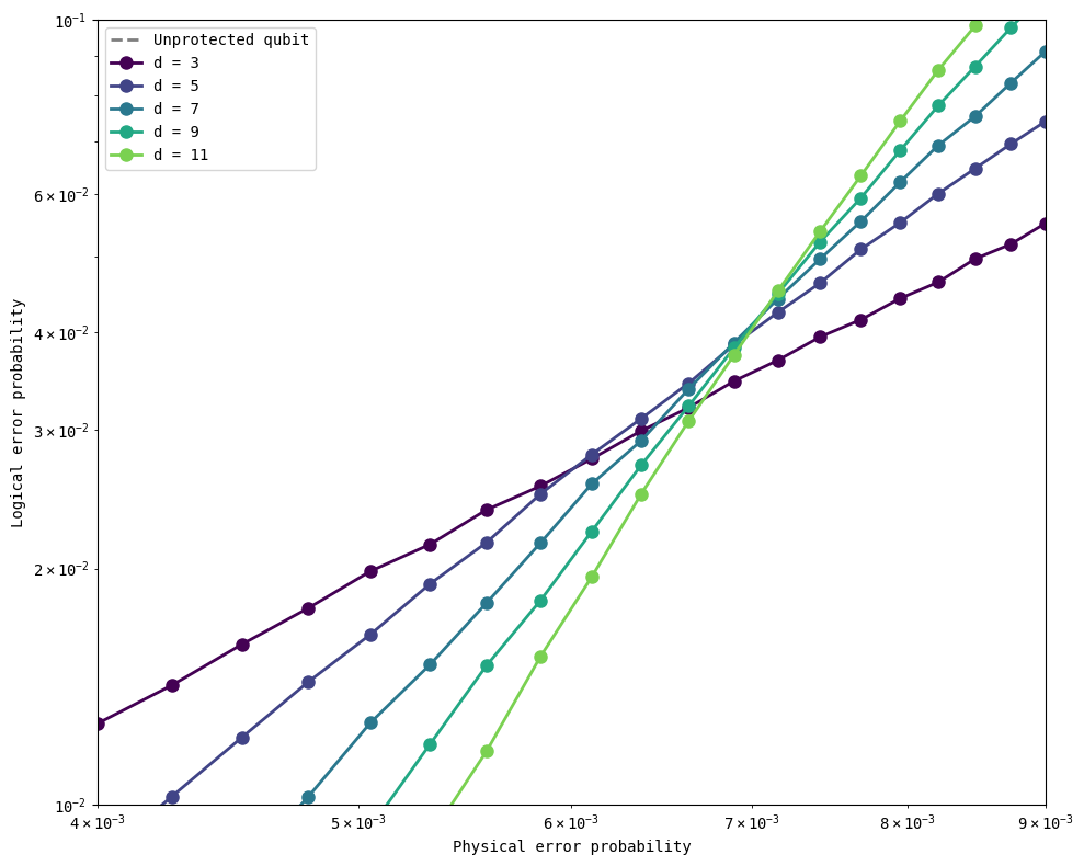
../../_images/d19d33eef42f5c39233745bf5d6298f2ba7204c9e9ca925f11809c80f257b924.png

As you see in the figure above, larger distances lead to lower logical error probabilities as the physical error probabilities go down. The curves for different distances cross over at about \(0.7\%\) error rate – this is close to the threshold for a surface code reported in the literature at about \(1\%\). In fact, we can rerun the simulations closer to that region to note the existence of multiple crossing points.

../../_images/31fcd29adff8ecdc7a9ee54b02b9279c0cea272075f7a7eb509007a61e8c09f6.png

Exercises for the reader

Can you identify reasons why the simulation doesn’t achieve a threshold closer to \(1\%\)? (Hint: consider the weights assigned to the various noise models in the simulation and compare them with those used in the literature).
Can you determine analytical expressions for the logical error probability as a function of distance and physical error probability for some of the noise models that stim provides?

Additional reading on the surface code and its threshold#

Version History#

v0: Aug 14, 2025, github/@ESMatekole
v1: Sep 12, 2025, github/@aasfaw