Reproducing repetition and Shor code simulations using stim#
So far, you have learned the structure of bit-flip and phase-flip repetition codes, and put them together in Shor’s 9-qubit code to protect against both kinds of errors. As you will see later, the lessons learned from these codes will extend into our discussion of surface codes.
To build and simulate the behavior of each of these error-correcting codes, you had to pay attention to:
The structure of the encoding and decoding circuits,
The stabilizers in use, and how the syndrome measurement circuits can be implemented,
How noise can be injected and used to detect when logical errors occur, and
The runtime of the simulations, and techniques for speeding them up by sampling efficiently.
State-of-the-art tools of the field like stim and Deltakit do all the above work for you, making it easy to produce the plots that we have seen so far. This chapter reproduces the results from bit-flip and phase-flip repetition codes, as well as the Shor code, in very few lines.
Introduction to stim#
The library stim [1] is able to generate the repetition code circuits that we have previously seen in one line, including insertion of noise. Here is an example that shows a distance-3 \(Z\)-type repetition code, where a specific type of depolarizing noise is inserted just before a round of syndrome measurements. Depolarizing noise is commonly used when exploring the error-correction performance of superconducting qubits.
distance = 3
error_probability = 0.1
c = stim.Circuit.generated("repetition_code:memory", distance=distance, rounds=1,
                           before_round_data_depolarization=error_probability)
display(c.diagram('timeline-svg'))

Note the resets at the beginning to initialize all qubits, including the distance data qubits (q0, q2 and q4), and distance - 1 auxiliary qubits (q1 and q3). Also note the measurements after the pairwise parity checks tagged rec[0] and rec[1].
One of the key features of stim is the use of detectors. A detector is a parity constraint on a set of measurement outcomes [2]. In the above circuit, there is one detector per check (parity check measurement) in each time slice, and these detectors compare that check’s outcome to the one before it. The very first detectors anchor the first check to the known start state after resets – without this, an error that happens before the first round (eg during reset) would not be detected. The very last detectors anchor the last checks to the end of the circuit – without this, a readout glitch in the last round would not be detected. The coordinates under the detectors are (x,t) pairs, indicating their space-time locations.
Altogether, a repetition code with distance data qubits running R rounds of syndrome checks would have (R - 1) \(\times\) (distance-1) between-round detectors, and then two more (distance-1) detectors anchoring to the start and end, for a total of (R + 1) \(\times\) (distance-1) detectors.
stim creates a rich detector error model that captures the effect of errors occuring at the various locations within the circuit, and assigns a weight to the probability of each of these errors flipping any of the detectors. This weighting can be used in a matching decoder to predict where errors might have occurred. stim also notes the effect of errors within the circuit on the observables tied to the circuit (\(Z_0Z_1Z_2\) in a distance-3 repetition code, for example), and the mismatch between the effect of an error on the observable and the prediction of a decoder can be used to determine logical errors.
Technical definitions of detectors, detection events, and detector error models (DEM)
\(\textbf{Definition 1: Detectors}\)
Stabilizer measurements are deterministic in the absence of errors. A detector is the parity of the measurement outcome bits in a QEC circuit. The outcome of a detector is 1 if the observed parity differs from the expected parity for a noiseless circuit, and is 0 otherwise. For example, a Pauli error \(\textbf{P}\) flips detector \(\textbf{D}\), if \(\textbf{P}\) acts non-trivially on the circuit, such that the measurement of \(\textbf{D}\) changes.
\(\textbf{Definition 1.1: Detection event}\) A detection event is a detector with outcome 1.
\(\textbf{Definition 1.2: Logical observables}\) A logical observable represents the outcome of logical operator. In general, logical observable measurement is non-deterministic. However, to benchmark the performance of a QEC code, we use experiments like quantum memory, where the outcome is deterministic as we know the encoded state. It is important to note that the decoder is unaware of the logical observable. It only receives the detector measurement outcomes.
\(\textbf{Definition 2: Detector error models}\)
Mathematical descriptions of the effects of errors on the QEC circuits. It is a way to track which errors can occur (depending on the noise model provided), how to detect these errors, and whether they caused a logical error. The detector error model can be understood as the representation of a parity check matrix or Tanner graph. It contains the information about the error mechanisms which connect the nodes representing the data qubits to the check nodes representing the auxiliary qubits.
\(\textbf{Definition 2.1: Detector error matrix (H)}\) The rows represent the detectors, and columns represent the possible error mechanisms such that; \(H_{i,j}=1\) if error mechanism \(j\) triggers detector \(i\) and \(H_{i,j}=0\) if error mechanism \(j\) does not affect detector \(i\).
\(\textbf{Definition 2.2: Logical observable matrix (L)}\) Similar to \(H\), the logical observable matrix \(L\) contains information whether an error mechanism affects the logical information.
Simulating bit-flip and phase-flip repetition codes using stim#
As in previous chapters, we will define a function get_logical_error_probability_for_rep_code which returns the logical error probability for a given configuration of distance and error_probability by sampling a number of shots. Then, we will repeatedly invoke this function for various parameters to generate the plots as we have previously done.
def get_logical_error_probability_for_rep_code(distance, p, basis="Z", rounds=1, n_shots=50_000):

    if distance == 1:
        return p

    circuit = stim.Circuit.generated(
        "repetition_code:memory",
        rounds=rounds,
        distance=distance,
        before_round_data_depolarization = 1.5*p, # note the factor of 1.5 here, discussion in footnote below
    )
    if basis == "X":
        # Switch basis from Z to X by applying global Hadamards
        # eg: H 0 1 2 3 4 for distance 5
        H_on_all_data_qubits = "H " + " ".join(str(qubit_index) for qubit_index in range(distance))
        circuit =   stim.Circuit(H_on_all_data_qubits) + \
                    circuit + \
                    stim.Circuit(H_on_all_data_qubits)

    # first, sample the circuit itself
    # we sample the circuit by creating a fast sampler that produces both detection events
    # and observable flips of the stabilizers without needing full statevector simulation
    # note that a detector is a parity check as we have been doing so far using auxiliary qubits
    # there are (d-1) * (R+1) detectors for distance d rep codes with R rounds corresponding to the pairwise ZZ/XX checks
    ds = circuit.compile_detector_sampler()
    # D = detector flips, shape (n_shots, n_detectors)
    # L = logical observable flips, shape (n_shots, n_observables)
    D, L = ds.sample(n_shots, separate_observables=True)

    # next, generate a decoder from the circuit's detector error model and use it to decode
    # the DEM maps possible error locations -> which syndrome parity checks (detectors) flip
    # and captures the probabilities of all the possible error locations (eg an X on qubit 1 after this specific gate)
    # leading to a flip of one of the detectors and logical observables
    dem = circuit.detector_error_model(decompose_errors=True)
    # the decoder is MWPM as we have seen so far, and the weights of the MWPM decoder come from the DEM's error probabilities
    m = pm.Matching.from_detector_error_model(dem)
    # then, use the decoder to predict when logical errors have occurred
    pred = m.decode_batch(D)

    # pred contains the error location predictions from the decoded syndrome measurements
    # L contains the actual observable flips
    # when the two mismatch, a logical error will occur
    total_logical_error_count = sum(pred[:, 0] != L[:, 0])

    return total_logical_error_count / n_shots
def get_logical_error_probability_stim(distances, ps, basis="Z", rounds=1, n_shots=50_000):
    p_Ls = np.zeros((len(distances), len(ps)))
    for i, d in enumerate(distances):
        print(f"Simulating distance-{d} repetition code circuits")
        for j, p in tqdm(enumerate(ps)):
            p_Ls[i, j] = get_logical_error_probability_for_rep_code(d, p, basis=basis, rounds=rounds, n_shots=n_shots)
    return p_Ls
Now, we can make our first physical error probability vs logical error probability study using stim using the above functions.
Bit-flip repetition codes#
ps = np.logspace(-4, -1, 20)
distances = [3, 5, 7, 9]
repcode_type = 'X'
n_shots = 30_000_000

p_Ls = get_logical_error_probability_stim(distances, ps, basis=repcode_type, rounds=1, n_shots=n_shots)
analytical_p_Ls = get_logical_error_probability_analytical(distances, ps)
plot_logical_error_probabilities(distances, ps, p_Ls, analytical_p_Ls, ylim = [1e-7, 1.1])
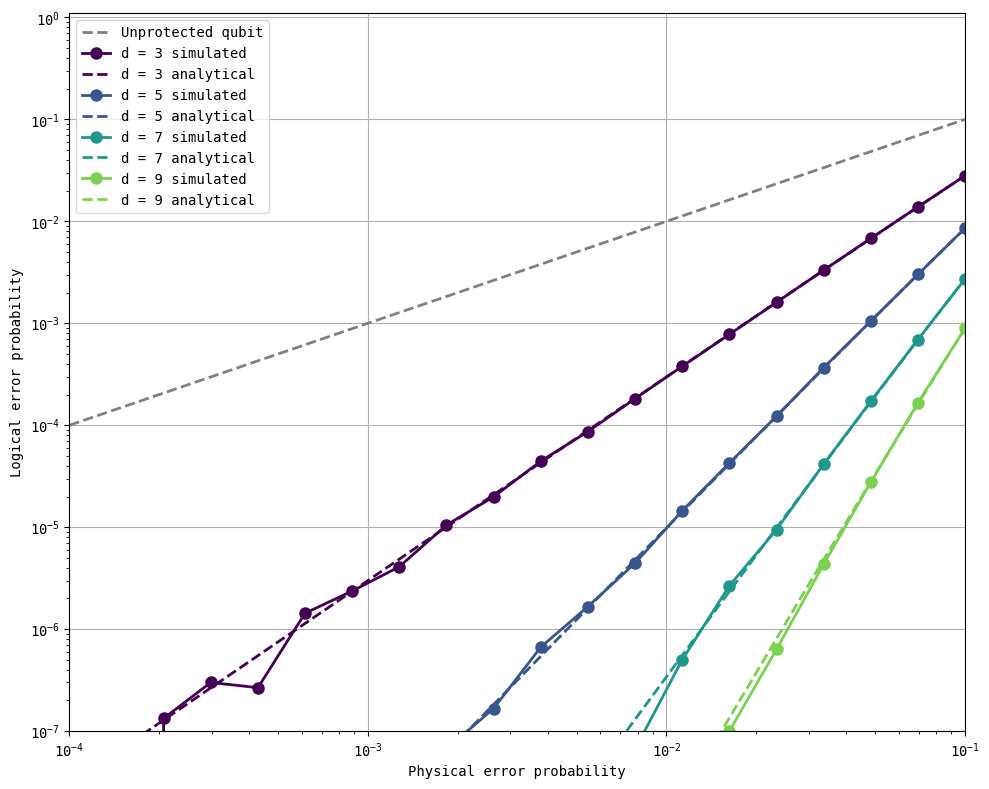
As you can see above, stim can sample 10 million shots in about 1 second at distance 3 with minimal use of the tricks in the previous chapter. To speed up these simulations even further by spreading the work across multiple CPU cores, another popular tool called sinter can be used.
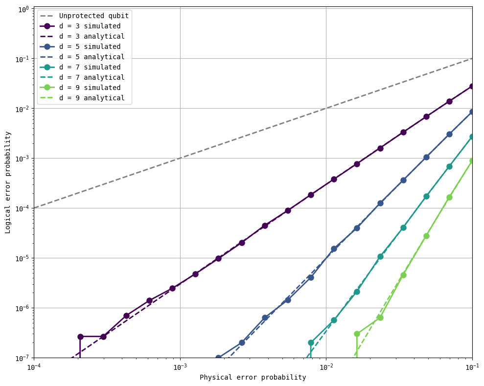
Phase-flip repetition codes#
ps = np.logspace(-4, -1, 20)
distances = [3, 5, 7, 9]
repcode_type = 'Z'
n_shots = 30_000_000

p_Ls = get_logical_error_probability_stim(distances, ps, basis=repcode_type, rounds=1, n_shots=n_shots)
analytical_p_Ls = get_logical_error_probability_analytical(distances, ps)
plot_logical_error_probabilities(distances, ps, p_Ls, analytical_p_Ls, ylim = [1e-7, 1.1])
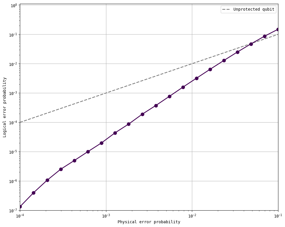
Simulating the 9-qubit Shor code using stim#
Since stim only provides circuit builders for repetition codes and surface codes, we will demonstrate how to define our own circuits below by building the Shor code.
def build_shor_code_circuit_stim(p, error_gate='X'):

    lines = []
    # prepare 3 GHZ blocks
    lines.append("R 0 1 2 3 4 5 6 7 8")
    lines.append("H 0 3 6")
    lines.append("CNOT 0 1 0 2 3 4 3 5 6 7 6 8")

    # insert error gates
    if error_gate == 'X':
        lines.append(f"X_ERROR({p}) 0 1 2 3 4 5 6 7 8")
    else:
        lines.append(f"Z_ERROR({p}) 0 1 2 3 4 5 6 7 8")

    # syndrome checks and associated detectors
    if error_gate == 'X':
        # X noise anti-commutes with ZZ checks within blocks
        for zz in ["Z0*Z1", "Z1*Z2", "Z3*Z4", "Z4*Z5", "Z6*Z7", "Z7*Z8"]:
            lines.append(f"MPP {zz}")
            lines.append("DETECTOR rec[-1]")
        # XX checks across blocks
        for xx in ["X0*X1*X2*X3*X4*X5", "X3*X4*X5*X6*X7*X8"]:
            lines.append(f"MPP {xx}")
            lines.append("DETECTOR rec[-1]")
        # Logical Z_L at the end (to be used as observable)
        lines.append("MPP Z0*Z3*Z6")
        lines.append("OBSERVABLE_INCLUDE(0) rec[-1]")
    else: # error gate is Z
        # Z noise anti-commutes with XX checks across blocks
        for xx in ["X0*X1*X2*X3*X4*X5", "X3*X4*X5*X6*X7*X8"]:
            lines.append(f"MPP {xx}")
            lines.append("DETECTOR rec[-1]")
        # ZZ checks within blocks
        for zz in ["Z0*Z1", "Z1*Z2", "Z3*Z4", "Z4*Z5", "Z6*Z7", "Z7*Z8"]:
            lines.append(f"MPP {zz}")
            lines.append("DETECTOR rec[-1]")
        # Logical X_L at the end (to be used as observable)
        lines.append("MPP X0*X1*X2*X3*X4*X5*X6*X7*X8")
        lines.append("OBSERVABLE_INCLUDE(0) rec[-1]")

    return stim.Circuit("\n".join(lines))

def get_logical_error_probability_for_shor_code(p, n_shots=50_000, error_gate='X', verbose = False):
    circuit = build_shor_code_circuit_stim(p, error_gate=error_gate)
    if verbose:
        display(circuit.diagram('timeline-svg'))

    # same workflow as in rep codes:
    # sample shots from the circuit to get detector and logical observable flips
    # create a DEM from the circuit to use for the decoder
    # determine if the decoder can use the detector flips to predict observable flips
    ds = circuit.compile_detector_sampler()
    D, L = ds.sample(n_shots, separate_observables=True)
    dem = circuit.detector_error_model(decompose_errors=True)
    m = pm.Matching.from_detector_error_model(dem)
    pred = m.decode_batch(D)
    total_logical_error_count = sum(pred[:, 0] != L[:, 0])
    return total_logical_error_count / n_shots

def get_logical_error_probability_stim_shor(ps, n_shots=50_000, error_gate='X'):
    p_Ls = []
    for j, p in enumerate(ps):
        if j == 0:
            p_Ls.append(get_logical_error_probability_for_shor_code(p, n_shots=n_shots, error_gate=error_gate, verbose = True))
        else:
            p_Ls.append(get_logical_error_probability_for_shor_code(p, n_shots=n_shots, error_gate=error_gate, verbose = False))
    return p_Ls
ps = np.logspace(-4, -1, 20)
n_shots = 30_000_000

p_Ls = get_logical_error_probability_stim_shor(ps = ps, n_shots = n_shots, error_gate = 'Z')
plot_logical_error_probabilities(None, ps, p_Ls, None, ylim = [1e-7, 1.1])

Further reading#
In this tutorial, you saw how stim can be used to reproduce the simulation results from the previous chapters. For further reading about stim, consider visiting the stim Github repository here. For further reading about PyMatching, consider visiting the PyMatching github repository here.
References#
Footnote: the astute reader may have noticed the factor of 1.5 that was inserted in the repetition code example (before_round_data_depolarization = 1.5*p). Until this chapter, \(p\) has signified the probability that an \(X\) or \(Z\) error is applied. The noise model used by stim with the setting before_round_data_depolarization=p applies \(X\), \(Y\) and \(Z\) errors, each with probability \(p/3\). In a \(Z\)-type repetition code memory experiment where we are trying to protect against bit-flip noise, both \(X\) and \(Y\) can cause bit-flips, but \(Z\) does not. So the effective bit-flip rate is \(p_{\text{flip}} = 2/3p\). To set the effective bit-flip rate to \(p\), we multiply by a factor of \(3/2=1.5\) as used in the example above. The same argument holds for \(X\)-type repetition codes.
Version History#
v0: Sep 12, 2025, github/@aasfaw
v1: Sep 16, 2025, github/@aasfaw edits capturing feedback from Earl Campbell