Lessons from classical error correction

Lessons from classical error correction#

Several of the key ingredients in quantum error correction can be intuitively understood by starting with the classical setting. In this chapter, we will walk through an example inspired by classical error correction. Throughout the discussion, we will demonstrate the results in Python.

A classical error correction scenario#

Imagine two parties (a sender and a receiver) communicating across a noisy channel. The effect of the noisy channel is to corrupt the communication between the two parties by introducing an error.

The sender transmits one bit (0 or 1) of information at a time, and the receiver gets each of those bits on the other side, but the noisy channel flips some of them from 0 to 1 (or vice versa).

To overcome the errors caused by the noisy channel, they agree on the simplest error-correcting protocol: let’s repeat the same message multiple times. The receiver then takes a majority vote of all the repeated bits to determine what the original message was. In error correction terminology, the two parties are communicating using a repetition code, with code distance equal to the number of times the message is copied/repeated.

Below, we write three functions to capture the communication between the two parties. The encode function creates num_copies copies of one bit of information. This is the message that the sender intends to transmit. Then, the send function takes those bits, and corrupts some of them with probability p_error by flipping them from 0 to 1 (or vice versa). Finally, the receive_and_interpret function takes in those bits and, depending on whether the majority_vote flag is set, returns either a single bit that won the majority vote, or the count of how many 0 and 1 bits were received.

def encode(bit, num_copies):
    return [bit] * num_copies

def send(bits, p_error = 0.1):
    return [1^bit if random.random() <= p_error else bit for bit in bits]

def receive_and_interpret(bits, majority_vote = False):
    received_bits_counted = Counter(bits).most_common()
    if majority_vote:
        return received_bits_counted[0][0]
    else:
        return received_bits_counted

Now, we can use these functions to demonstrate the key ingredients of error correction.

For example, we can encode the message 1 repeatedly by writing

message = encode(1, 5)
print(message)

[1, 1, 1, 1, 1]

We can then transmit this message across a noisy channel by writing

transmitted = send(message, p_error = 0.1)
print(transmitted)

[1, 1, 1, 1, 1]

And finally, we can interpret what these bits could have meant by writing

received = receive_and_interpret(transmitted)
print(received)

[(1, 5)]

where we see how many 0s and 1s were received, or take a majority vote by writing

received = receive_and_interpret(transmitted, majority_vote = True)
print(received)

Measuring the effectiveness of classical repetition codes#

Now, let’s ask the following question: how well does this duplicate-and-take-majority-vote scheme work?

To do this, we run several iterations (n_shots) where we send a randomly picked message across the channel to see when we can successfully recover the desired message. We will count the number of times we are unable to recover the desired message, and report it as a probability in n_shots attempts.

def get_code_error_probability(code_distance, p_error, n_shots = 1000):

    code_errors = 0.0
    for _ in range(n_shots):
        desired_message = random.choice([0,1])

        encoded_message = encode(desired_message, num_copies = code_distance)
        sent_message = send(encoded_message, p_error = p_error)
        received_message = receive_and_interpret(sent_message, majority_vote = True)

        if received_message != desired_message:
            code_errors += 1

    return code_errors / n_shots

We will try several code distances to see the impact of increasing the code distance. Note that we are only using odd-numbered distances $(1,3,5,\ldots)$ so that we can ensure that majority voting works.

code_distances = np.arange(start = 1, stop = 21, step = 2)
p_errors = np.logspace(start = -3, stop = 0, num = 50)

all_code_distance_error_probabilities = []
for code_distance in code_distances:
    print(f"Running distance {code_distance}")
    code_distance_error_probabilities = []
    for p_error in p_errors:
        code_distance_error_probabilities.append(
            get_code_error_probability(code_distance, p_error, n_shots = 100000)
        )
    all_code_distance_error_probabilities.append(code_distance_error_probabilities)

Running distance 1
Running distance 3
Running distance 5
Running distance 7
Running distance 9
Running distance 11
Running distance 13
Running distance 15
Running distance 17
Running distance 19

Now, we can plot the results to see the effectiveness of the error-correcting scheme.

for code_distance, error_probabilities in zip(code_distances, all_code_distance_error_probabilities):
    plotter.loglog(p_errors, error_probabilities, marker = '.', markersize = 10, label=f'd = {code_distance}')
plotter.legend()
plotter.xlabel('Per-bit error probability')
plotter.ylabel('Message error probability')
plotter.xlim([1e-3, 1.1])
plotter.ylim([1e-3, 1.1])
plotter.grid()
plotter.show()

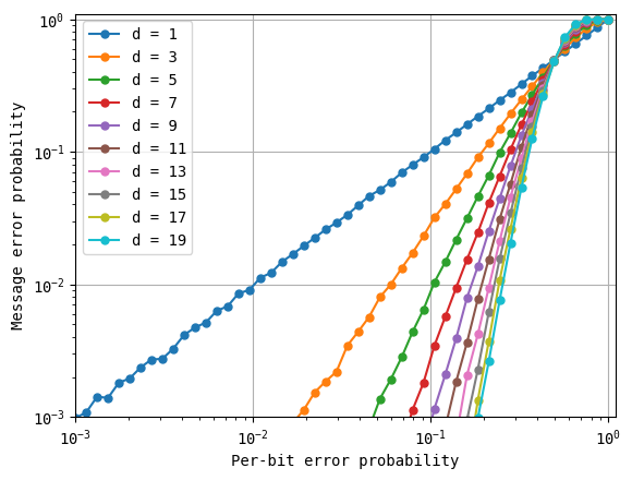
../../_images/9c21d02230323734efc94be8c9541713818bf732fff937eaea1da7083bb5ceb5.png

First, note that code distance d = 1 has no effect on the message. When the probability of error introduced by the channel (the x-axis labeled per-bit error probability) is $10^{-2}$, so is the probability of error of the encoded message (the y-axis labeled message error probability). However, for larger distances, a reduction in the per-bit error probability leads to steeper reductions in the error of the encoded message. For example, at distance $3$, the same per-bit error probability leads to an error in the received message that is well below $10^{-3}$, a 10x improvement.

To see the effect of error correction more clearly, we take a vertical slice of the above plot for a specific value of per-bit error probability, and see what happens at various code distances.

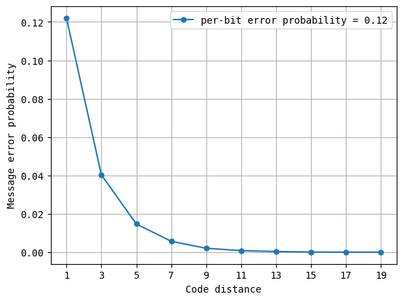
../../_images/a063fd128e574d16d41cb26f8ba626b237583de0c8cfe1829053241ffeee5af4.png

As you can see, increasing code distances result in an exponential suppression of the per-bit error. For the specific value of p_error = 0.12, the error of the message being misinterpreted is already down 3x at code distance 3, and $\sim8$x at code distance 5.

The presence of a threshold#

The astute reader may have noticed in the above plots that error correction makes things worse (and not better) when the per-bit error is large. We can see this more clearly by replotting as shown below.

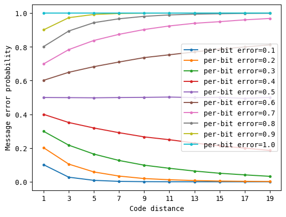
../../_images/645d378600790e8ab57e04ce02b4ca1d892d830cf4aebc2a5d1b20ac11aef5e7.png

As you can see above, as the per-bit error probability crosses $0.5$, the effect of our error correction scheme flips. When the noisy channel is simply too noisy (and therefore the per-bit error probability is larger than $0.5$), error correction doesn’t help at all – in fact, it makes things worse because each redundantly added bit is unlikely to help the situation. However, when the noisy channel is good enough (with a per-bit error probability less than $0.5$), the benefits of our error correction scheme appear clearly, resulting in an improvement in chance of success that the received message is interpreted successfully. The specific value of the per-bit error probability where the effect of error correction flips sharply is known as the threshold. From an engineering standpoint, we want to create a noisy channel that is at least that good, so that we can employ error correction and achieve low overall errors.

The challenge of correlated errors#

So far, the kind of error mechanism we simulated was a random flip of each bit, independently of what happens to all other bits. In the language of statistics, this is known as an independent, identially distributed (i.i.d.) noise model – each bit in the repetition code has no “knowledge” of what happened to all the others, and experiences the error independently on its own.

Error correction can handle these kinds of errors easily using schemes like the repetition code. However, when there is some correlation in the way that the bits experience the noise – for example, two bits will always flip at the same time – then the effectiveness of a repetition code is limited. In this section, we will demonstrate this effect by writing down two noise models and running the same simulations above.

The correlated noise model that we will use is inspired by experimental observations of error bursts due to cosmic rays (see McEwen et al, arxiv:2104.05219). When these events occur (sometimes due to energy impacts from cosmic rays), the quantum processor experiences errors across all qubits. We will model this scenario as follows: with a small probability $p_\text{correlated}$, all bits in our repetition code will flip. Otherwise, each of the bits will flip independently as before with probability $p_\text{error}$.

def send_with_random_iid_bitflip(bits, p_error = 0.1):
    return [1^bit if random.random() <= p_error else bit for bit in bits]

def flip_all_bits(bits):
    return [1^bit for bit in bits]

def send_with_correlated_bitflip(bits, p_error = 0.1, p_correlated = 1e-4):
    # with probability p_correlated, flip all bits
    #otherwise, flip each bit independently with probability p_error
    if random.random() <= p_correlated: # flip every bit
        return flip_all_bits(bits)
    else:
        return send_with_random_iid_bitflip(bits, p_error)

code_distances = [3, 7, 13]
p_errors = np.logspace(start = -6, stop = 0, num = 30)
p_correlated = 2e-4

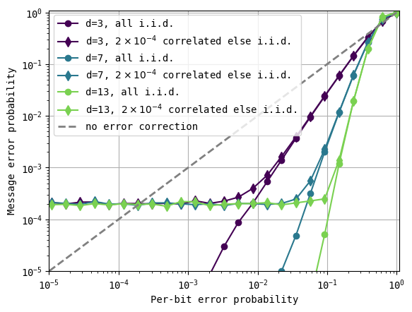
../../_images/cc54573825d3a986c7f5615d59d176255a9eb1f67feb01cc026f5345c3a555a9.png

As you can see above, even small amounts of correlated errors that break the indepedent, identically distributed noise model assumption can lead to a catastrophic outcome. No matter how low the error of flipping individual bits gets, the benefit of error correction remains limited to a level determined by the correlated errors. Perhaps more importantly, no matter how large of a code distance we go to, the logical error probability never gets lower, highlighting that deploying “more” error correction by increasing the size of the repetition code does not help. The only way out is to resolve the cause of the error bursts, or to shield from them in the experimental setting when possible. For the specific example discussed above with superconducting qubits, the authors have identified one solution that resists high-energy impacts by modifying the fabrication techniques of the processors (see McEwen et al, arXiv:2402.15644).

Exercise for the reader

We used the majority vote decoder to interpret the received message above. This decoder only works when $p < 0.5$ such that most bits remain unflipped. When $p > 0.5$, there exists another decoder that works. Can you identify that decoder? How would you modify the majority vote decoder to implement it?

Easter egg

The first plot in this chapter (message error probability vs per-bit error probability) appears on the cover page of the textbook. However, note that the plot on the cover has a y-axis that extends to the $10^{-9}$ (part-per-billion) range. Doing this requires taking a few billion shots of statistics. This takes a lot of time to do, but you will learn the techniques to speed up these simulations later in this textbook (see the chapter on running faster circuit simulations).

Version History#

v0: Sep 12, 2025, github/@aasfaw
v1: Sep 16, 2025, github/@aasfaw edits capturing feedback from Earl Campbell